Project Part 2

Interactive and static plots of drug deaths from 2010 to 2019

Part 2

1. Packages that I will use to read in and plot the data:

library(tidyverse)
library(echarts4r)

2. Read the data in from Part 1:

regional_drugdeaths <- read_csv(here::here("regional_drugdeaths.csv"))

Interactive Graph

• Start with the data
• Group_by region so there will be a “river” for each region
• Use mutate to round DeathsfromDrugUse so only 2 digits will be be displayed when you hover over it
• Use mutate to change Year so it will be displayed as end of year instead of beginning of year
• Use e_charts to create an e_charts object with year on the x axis
• Use e_river to build “rivers” that contain DeathsfromDrugUse by region. The depth of each river represents the amount of deaths for each region
• Use e_tooltip to add a tooltip that will display based on the axis values
• Use e_title to add a title, subtitle, and link to subtitle
• Use e_theme to change the theme to roma

regional_drugdeaths %>%
  group_by(Region) %>%
  mutate(DeathsfromDrugUse = round(DeathsfromDrugUse, 2),
         Year = paste(Year, "12", "31", sep="-")) %>%
  e_charts(x = Year) %>%
  e_river(serie = DeathsfromDrugUse, legend = FALSE) %>%
  e_tooltip(trigger = "axis") %>%
  e_title(text = "Annual Drug Deaths, by World Region",
          subtext = "(per 100,000 people). Source: Our World in Data",
          sublink = "https://ourworldindata.org/illicit-drug-use#deaths-from-drug-use-disorders",
          left = "center") %>%
  e_theme("wonderland")

Static Graph

• Start with the data
• Use ggplot to create a new ggplot object. Use aes to indicate that Year will be mapped to the x axis; DeathsfromDrugUse will be mapped to the y axis; Region will be the fill variable.
• geom_area will display DeathsfromDrugUse
• scale_fill_discrete_divergingx is a function in the colorspace package. It sets the color palette to Wonderland and selects a maximum of 12 colors for the different regions
• theme_classic sets the theme
• theme(legend.position = "bottom") puts the legend at the bottom of the plot
• labs sets the y axis label, fill = NULL indicates that the fill variable will not have the labeled Region

regional_drugdeaths %>%
  ggplot(aes(x = Year, y = DeathsfromDrugUse, fill = Region)) +
  geom_area() +
  colorspace::scale_fill_discrete_divergingx(palette = "ArmyRose", nmax = 12) +
  theme_classic() +
  theme(legend.position = "bottom") +
  labs(y = "per 100,000 people",
       fill = NULL)

ggsave(filename = "preview.png",
       path = here::here("_posts", "2022-05-15-project-part-2"))

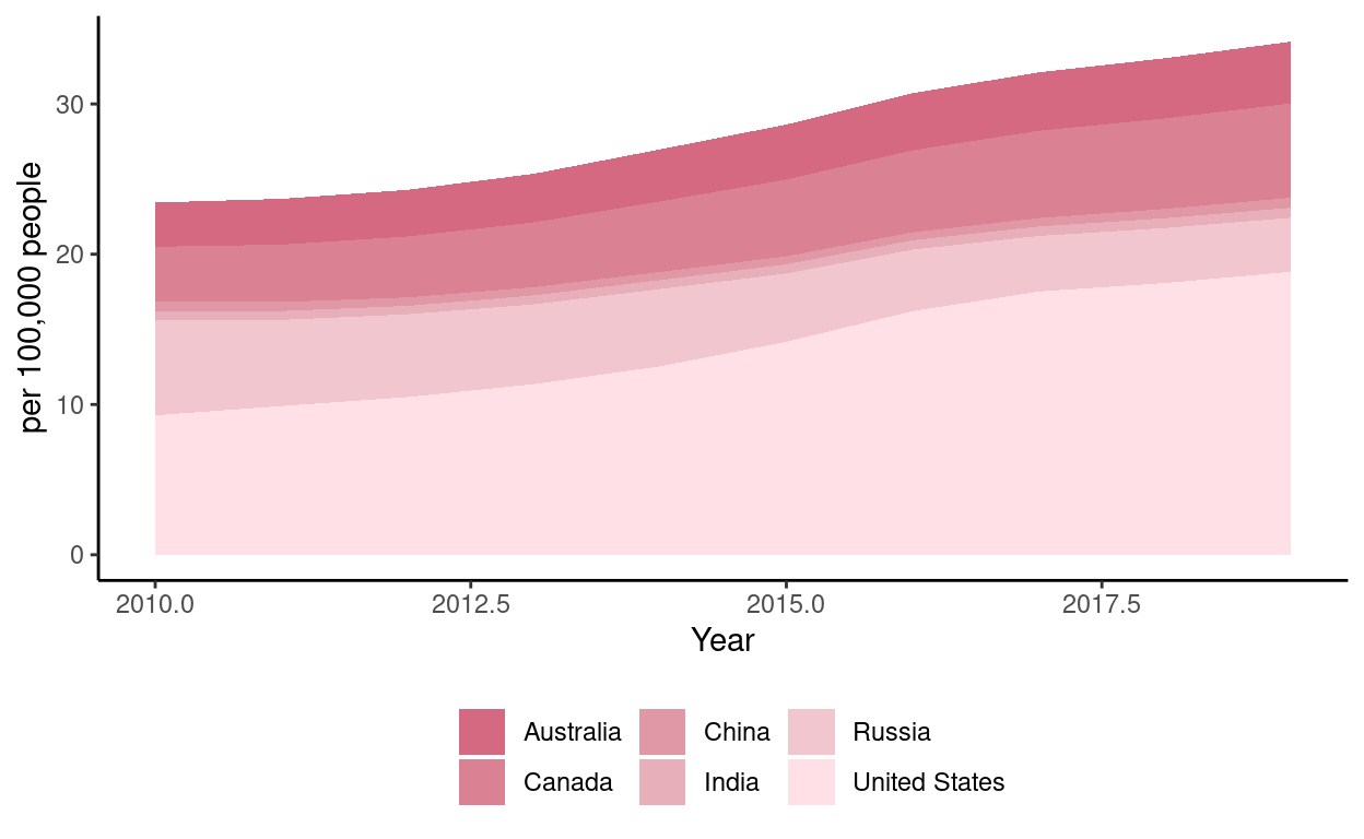
These plots show that the United States has been the leader in deaths from illicit drug use. Since 2010, deaths have continued to increase at a rapid rate. Deaths in 2019 were double what they were in 2010.