Sampling

Based on Chapter 7 of ModernDive. Code for Quiz 11.

1. Load the R packages we will use.

library(tidyverse)
library(moderndive)

2. Quiz questions.

Question:

7.2.4 in Modern Dive with different sample sizes and repetitions

• Make sure you have installed and loaded the tidyverse and the moderndive packages
• Fill in the blanks
• Put the command you use in the Rchunks in your Rmd file for this quiz

---

Modify the code for comparing different sample sizes from the virtual bowl

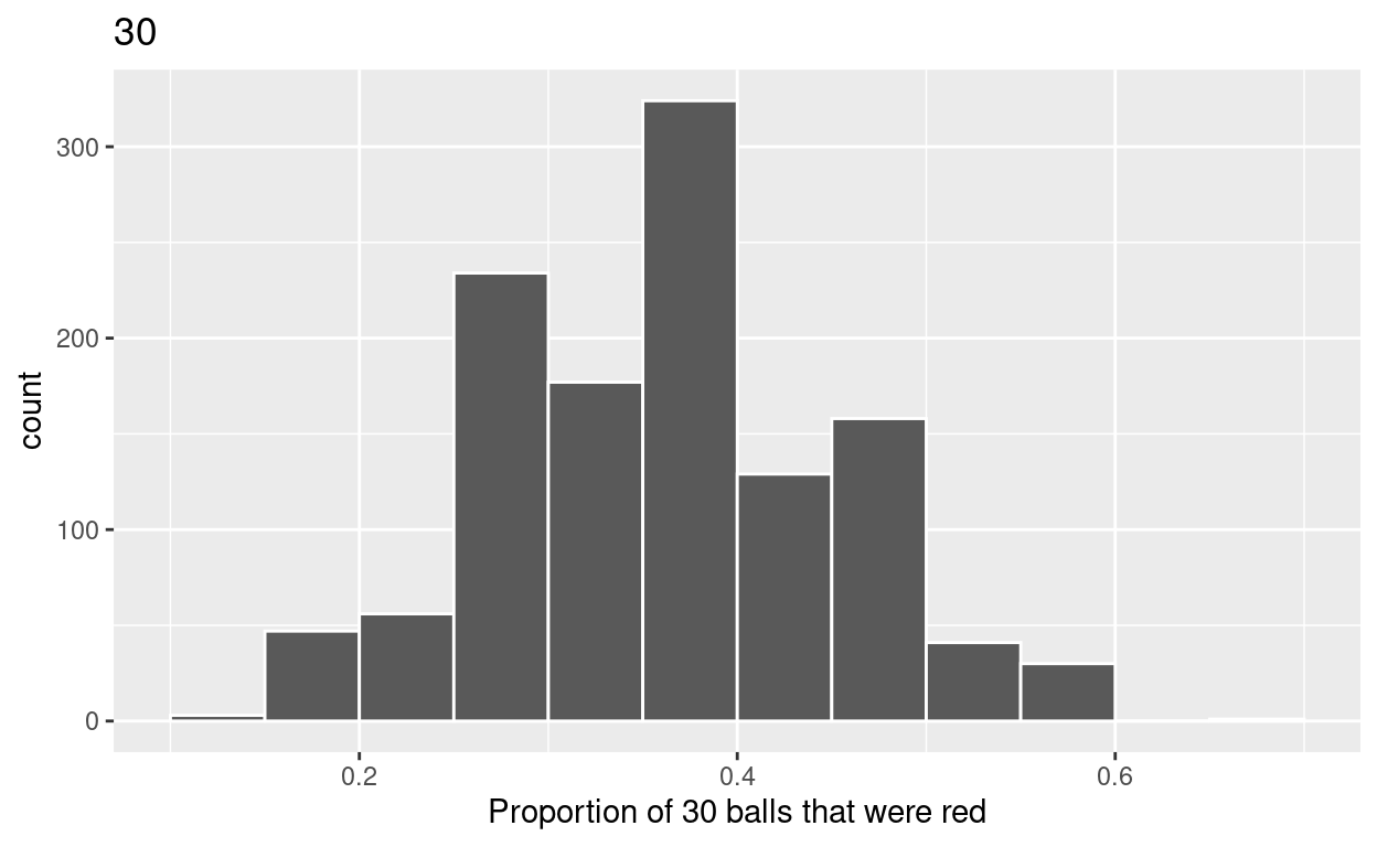
Segment 1: sample size = 30

1. a. Take 1200 samples of size of 30 instead of 1000 replicates of size 25 from the bowl dataset. Assign the output to virtual_samples_30.

virtual_samples_30  <- bowl  %>% 
rep_sample_n(size = 30, reps = 1200)

2. Compute resulting 1200 replicates of proportion red.

• start with virtual_samples_30 THEN
• group_by replicate THEN
• create variable red equal to the sum of all the red balls
• create variable prop_red equal to variable red / 30
• Assign the output to virtual_prop_red_30

virtual_prop_red_30 <- virtual_samples_30 %>% 
  group_by(replicate) %>% 
  summarize(red = sum(color == "red")) %>% 
  mutate(prop_red = red / 30)

3. Plot distribution of virtual_prop_red_30 via a histogram. Use labs to

• label x axis = “Proportion of 30 balls that were red”
• create title = “30”

ggplot(virtual_prop_red_30, aes(x = prop_red)) +
  geom_histogram(binwidth = 0.05, boundary = 0.4, color = "white") +
  labs(x = "Proportion of 30 balls that were red", title = "30") 

---

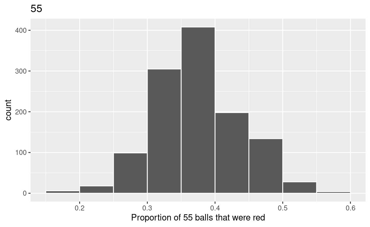
Segment 2: sample size = 55

2. a. Take 1200 samples of size of 55 instead of 1000 replicates of size 50. Assign the output to virtual_samples_55.

virtual_samples_55 <- bowl  %>% 
rep_sample_n(size = 55, reps = 1200)

2. Compute resulting 1200 replicates of proportion red.

• start with virtual_samples_55 THEN
• group_by replicate THEN
• create variable red equal to the sum of all the red balls
• create variable prop_red equal to variable red / 55
• Assign the output to virtual_prop_red_55

virtual_prop_red_55 <- virtual_samples_55 %>% 
  group_by(replicate) %>% 
  summarize(red = sum(color == "red")) %>% 
  mutate(prop_red = red / 55)

3. Plot distribution of virtual_prop_red_55 via a histogram. Use labs to

• label x axis = “Proportion of 55 balls that were red”
• create title = “55”

ggplot(virtual_prop_red_55, aes(x = prop_red)) +
  geom_histogram(binwidth = 0.05, boundary = 0.4, color = "white") +
  labs(x = "Proportion of 55 balls that were red", title = "55") 

---

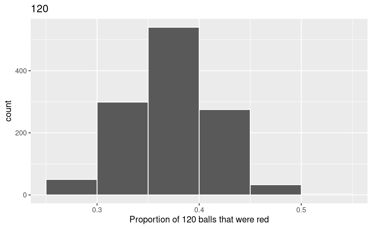
Segment 3: sample size = 120

3. a. Take 1200 samples of size of 120 instead of 1000 replicates of size 50. Assign the output to virtual_samples_120.

virtual_samples_120  <- bowl  %>% 
rep_sample_n(size = 120, reps = 1200)

2. Compute resulting 1200 replicates of proportion red.

• start with virtual_samples_120 THEN
• group_by replicate THEN
• create variable red equal to the sum of all the red balls
• create variable prop_red equal to variable red / 120
• Assign the output to virtual_prop_red_120

virtual_prop_red_120 <- virtual_samples_120 %>% 
  group_by(replicate) %>% 
  summarize(red = sum(color == "red")) %>% 
  mutate(prop_red = red / 120)

3. Plot distribution of virtual_prop_red_120 via a histogram. Use labs to

• label x axis = “Proportion of 120 balls that were red”
• create title = “120”

ggplot(virtual_prop_red_120, aes(x = prop_red)) +
  geom_histogram(binwidth = 0.05, boundary = 0.4, color = "white") +
  labs(x = "Proportion of 120 balls that were red", title = "120") 

ggsave(filename = "preview.png",
       path = here::here("_posts", "2022-04-19-sampling"))

---

Calculate the standard deviations for your three sets of 1200 values of prop_red using the standard deviation

n = 30

virtual_prop_red_30 %>%
  summarize(sd = sd(prop_red))

# A tibble: 1 × 1
      sd
   <dbl>
1 0.0903

n = 55

virtual_prop_red_55 %>%
  summarize(sd = sd(prop_red))

# A tibble: 1 × 1
      sd
   <dbl>
1 0.0626

n = 120

virtual_prop_red_120 %>%
  summarize(sd = sd(prop_red))

# A tibble: 1 × 1
      sd
   <dbl>
1 0.0415

The distribution with sample size, n = 120, has the smallest standard deviation (spread) around the estimated proportion of red balls.